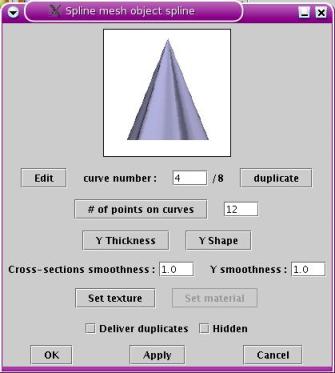
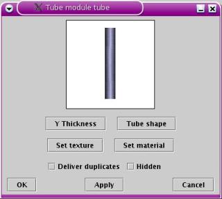
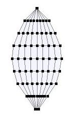
The Tube shape button allows to
edit the tube like an ordinary AoI tube. Usually, though, you would set
the thickness of the tube for individual points (or a selection of
them). The TaPD tube uses a customised function, exactly like the
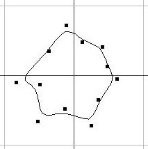
spline mesh object. This function is defined using the R Shape button. Like for the spline
mesh object, the tube control points define the resolution of the Y
curve of the tube object. Any consideration discussed in the spline
mesh object section are valid for the tube object, except of course
those addressing cross-sections.
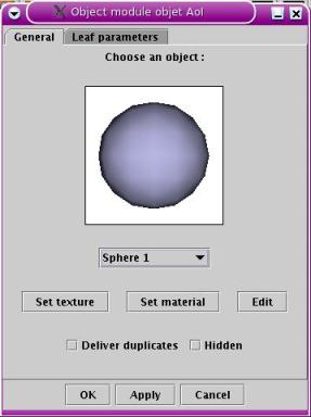
Set texture and Set material allow to assign texture
and material to the tube (the ends of which are flat).
The Deliver duplicate
and Hidden checkboxes works
the same way as for the AoI object module discussed
earlier.
Tube objects use much less memory (and rendering time) than spline mesh
objects. Hence, they should be preferred to spline mesh objects
whenever possible.
3.2
Geometry modules
All
geometry modules show a maroon background. They always have at least
one object input and one object output. There are two kinds of geometry
modules :
- Modules
that only have one object input and one object output. These could be
classified as 'neutral' and do not create any object to be added to the
object collection the TaPD object is made of. They can modify an object
(Distort module) or simply
influence the way the procedure works (Random
module).
- Modules
that have two object input ports and one object output port. These
modules decorate an object with copies of another object which is
called the decorator object. A typical example of a decorator module is
the Coil module, which is the module that is described below.
3.2.1 Coil
module 

The coil module
is the current keystone of the geometry modules. It is by far the
most complicated module that can be used in a procedure. Its function
is to place and orientate decorator objects along an object to
decorate. The decoration process takes place along the vertical axis of
the decorated object much like a spiral staircase. At each step of the
"stair", a decorator object may be placed along the decorated object
depending on a probability check. Depending on parameters used in the
coil module, the decorated object can be distorted during the process.
The decorated object may also be distorted due to "counter reaction"
effects which are also setup in the module.
The use of the coil module is typically to decorate a trunk with
branches or decorate branches with smaller branches or leaves.
There is also a special mode that uses the golden ratio to place the
decorator object. In this mode, decorators positions do not follow the
"spiral staircase" scheme anymore. See the special section devoted to
the use of the golden ratio decoration.
Input / Output :
The first entry port (the left port using the default I/O layout)
corresponds to the input of the object to be decorated. The second port
(on the top) corresponds to the decorator object input. The object
output port
makes it possible to plug the decorator object to other modules which
may in turn decorate the decorator object. This recursive process
allows to create fractal objects, a common feature for trees and
plants. There are three value input ports. The first one allows to
enter an Y value used for specified customized functions to compute
parameters based on the entered value (more anout that later on, it's
rather an advanced topic). The two other bottom input ports allow to
plug constant values or
(much more frequently) customised functions that will govern size
variation
of the decorator objects (both in width and height) along the Y axis of
the decorated object. All examples shown belown were obtained using a
default customised funtion plugged into both R and Y size inputs.
Finally, the Y output port makes it possible to redirect the current Y
value of the coil module into a value input port, presumably the Y
value input port of another coil module or a golden ball module.
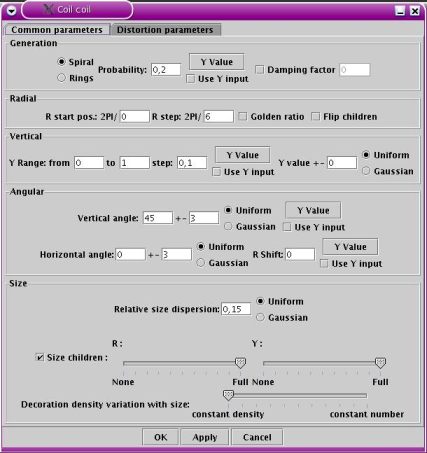
The edit window dialog consists in two parameter panes. The first pane
concerns basic geometric parameters that work for any
decorated/decorator object type, be it AoI object or TaPD objects
(spline mesh and tube). The second pane is relevant only if the
object used as decorator (or, in the counter-reaction effect case, used
as decorated object) is a proper TaPD object or a planar spline mesh
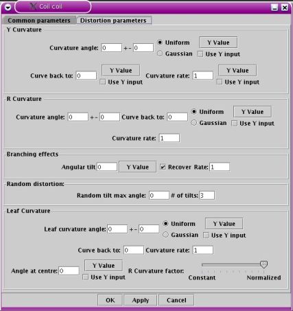
used to model leaves. The figure below shows
the first pane of the edit window of a coil module :

First pane of the coil module edit
window
The parameters shown in this pane are explained below. The basic
process of the coil module is the following :
- Start
from a given position and orientation along the vertical axis of the
decorated object;
- Check if
a decorator object has to be placed there;
- Increment
and repeat until the top of the object is reached.
Positions along
the vertical axis are referred to as Y positions and range from 0 (the
bottom of the decorated object) to 1 (the top of the decorated object).
This coordinate is a so-called reduced coordinate : it ranges from 0 to
1 whatever the real height of the decorated object.
Orientations of the decorator objects whithin the radial plane
(cross-sectional plane) of the decorated object are referred to as R
positions. They are usually expressed in degrees, sometimes as 2PI/n,
where n is an integer.
Incrementing both Y and R values step after step and placing decorator
objects yields the staircase (or screw) geometry created by the coil
module.
Spiral / Rings : Spiral means that
at each R step, the Y value of the decorator position is increased. A
spiral staircase layout is then obtained. Rings mean that Y positions
are incremented only after the R position of the decorator object has
gone one full turn. In that case, rings of decorator object along the
vertical axis of the decorated object are obtained.
Probability : This float number
between 0 and 1 is the probability that a decorator object is placed at
each possible position. A value of 0 means that no decorator object is
ever placed on the decorated object, a value of 1 (100%) means that all
possible positions are occupied.
Y Value button : Clicking this
button brings an editor window which is a customized function editor
taken from the procedural texture editor. This function is used to vary
the probability value along the Y axis of the decorated object. The
probability value at some Y position of the decorated object is
evaluated as :
overall value
= constant probability value x function
value (Y)
Y ranges from 0 (bottom) to 1 (top).
Supposing you want more decorators at the top of the object than at the
bottom, you could use a customized function that starts at 0.5 (for
example) and reaches 1 for x=1. Every parameter that shows an Y Value
button near the text entry can be varied along the Y axis the same way.
Use Y input checkbox : This option
is used to determine whether the Y value considered for evaluation of
the customised function value as described in the Y Value button section is internal
or external. Usually, you would use the internal Y value of the module,
i.e. the current height along the Y axis of the decorated object, to
vary the probability (or some other parameter that uses the Y Value mechanism). There are some
times, however, when you want to use a value that is input in the Y
input port. Let us suppose that you want to design a flower that is
made of a primary stem, secondary stems that decorate the main stem
through use of a coil module named coil#1, and flowers on top of the
secondary stems. The petals the flowers consist of are places using a
coil#2 module. Let us also suppose that you want the petals of the
flower to 'close' as the secondary stems are placed towards the top of
the main stem. Using the usual internal Y value to vary the vertical
angle won't help, since petals are always put at the top (1.0) of the
secondary stems. But if you plug the Y output value port of the coil#1
module into the Y input value port of the coil#2 module and activate
the Use Y input checkbox option for the
vertical angle customised function, then you can vary the vertical
angle parameter as needed.
Damping factor : Experimental
parameter that will remain in the TaPD if its proven useful. The
problem of random occupation of the decorator positions is that you
could get three decorator objects in a row and then nothing for the ten
subsequent positions. The damping factor (an integer d ) tries to attenuate this effect
by lowering the probability right after a decorator has been
successfully placed. The new probability is then probability /d , the next step it
is evaluated as probability /(d-1) and so forth for
each unsuccessfull step until it reaches its usual value. The primary
use of the damping factor is to fine tune decoration. Quite logically,
the density of decorators decreases as the damping factor increases. If
you end up with a high damping factor, it is likely that the geometric
parameters used should be modified.
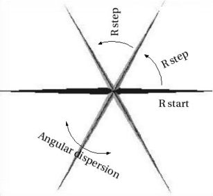
R start : this integer parameter
represents the radial angular origin at which the decoration process
begins (see figure coil.1a). It is expressed as 2PI/n, n=0 having
a special meaning : the origin is then 0. Usually, this parameter does
not need to be modified, except when two coil modules are merged. In
that case, it is customary to use a non zero integer for n so that the
two
coil modules do not place decorator objects at the same radial angular
position. You may also use the same radial origin but different Y start
parameters (see further description of this parameter) to avoid
overlapping of decorator objects.
R step : this integer parameter
represents the radial angular step separating each possible positions
of the decorator objects (see figure coil.1a below). Once again, it is
expressed as 2PI/n.
Golden ratio : if this option is
enabled, the decoration process uses a special golden section rule. See
end of module description.
Flip children : If you use leaves
that show an 'up' side and a 'down' side (different front and back
texture, or leaf distorsion) for horizontal branch decoration, the
default decoration process is such that leaves placed at R=PI/4 or
45° will show their up side globally facing towards the sky whereas
the leaves placed at R=3PI/2 or 270° will have their up sides
facing towards the ground. Activating this option causes every
decorator placed at 180<R<=360° to be flipped to keep correct
orientation. There is no mechanism (yet) to globally reorientate leaves
towards the sky once the plant or tree is build.

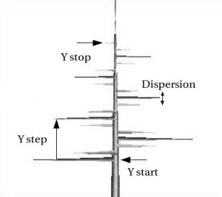
figure coil.1.a
|

figure coil.1.b
|
Y start : this value is the Y
position where the decoration process begins. It is expressed in reduce
coordinates, from 0 (bottom) to 1
(top). See figure coil.1.b.
Y stop : this value is the Y
position where the decoration process ends. See figure coil.1.b.
Y step : the increment in Y after
each turn in R. This value can be varied along the Y axis using the Y value button.
+- : If a decorator object is
successfully placed at a given position, the Y coordinate can be
randomised by an amount corresponding to a random distribution
comprised between +value and -value. The random distribution can be
uniform or gaussian. Uniform distributions are used to randomise the
decoration process so that it does not lead to a "too geometrically
perfect" object. The gaussian distribution purpose is different : let's
suppose you are modeling a plant which places its leaves every 2PI/4
(90°) in R along the stem. Most certainly, the leaves aren't
exactly places every 2PI/4. There will be some deviation, even some
accidents for a few leaves for which the angle might get to 80° or
100°. Using the uniform random distribution do not make it possible
to reproduce that behaviour : all angular positions will be uniformly
scattered whithin the width of the distribution. The gaussian
distribution, however, yields angular values close to the perfect one,
but for a few positions that will show anomal deviation. Therefore, a
rule of thumb for choosing between uniform or gaussian is :
- if you
want to randomise decorator positions to "hide" the coil module
parameters used, use a uniform distribution.
- if
you model a plant that has well defined geometric parameters, use the
gaussian distribution to simulate natural imperfections.
Vertical angle : This parameter
represents the angle between the vertical axis of the decorated object
and the vertical axis of the decorator object. 90° corresponds to a
right angle between the two objects. This parameter can be varied along
the height of the decorated object using the Y value button. The value of the
angle can be randomised by a certain amount, entered in the +- text entry, and using a uniform
or gaussian distribution as explained before.
Horizontal angle : This parameter is
strictly equivalent to the R angular position, so in fact it's
redundant and will probably be removed. Keep the default null value.
The +- text entry, however, is important
since it allows to randomise the angular positions. For example,
looking at figure coil.1.a, it's obvious that these angular positions
do not fit for modeling a tree. In fact, angular positions should be
randomised by a uniform distribution having a width of 2PI/6 = 60°,
so a value of +-30° is sensible. Using lower values for the
distribution width can avoid having angular positions being too close
to each other, so a value of 20°, for example, might be preferred.
R shift : By default, the coil module places the decorator
objects right along the Y axis of the decorated object. If the
decorator object is small, it might not even show through the decorated
object ! The R shift parameter allows to shift radially the decorator,
so that its base lies at the surface of the decorated object. For a
TaPD decorated object, this value should be about half the R size of
the decorator (difference between a radius (R shift) and a diameter
(object module R size)). The customised function accessed through the Y value button should reproduce the
shape of the decorated object. The R Shift algorithm takes care of
radial resizings of children that might have occured in previous coil
modules. This parameter is typically useful for decorating an object
with needles. Warning : If the R shift parameter is used for objects
having a small radius (say 0.05), the preview windows might show a gap
between decorated object / decorator objects. This is not a bug in the
TaPD : it's just the precision of the preview window that is too low.
There is nothing to worry about, but the necessary precision for
rendering must be specified if theis phenomenon happens also in
rendered images.
Relative size dispersion : The size
variation along the Y axis of the decorated object is taken from the
value inputs. However, it can assumed that the sizes of the decorator
objects have
to vary randomly as well. The relative size dispersion parameter states
by which amount the randomisation affects the sizes of the decorators.
A value of 0.1 (10%) means that the size will vary between 90% and 110%
of the original object to which the size input values have been applied.
Size children : This option is quite important. Let's consider a
coil module, the function of which is to decorate branches (placed by a
former coil module around a trunk) with other branches. We will suppose
that these branches have been scaled by the first module along the Y
axis of the trunk. The second coil module must take into account the
size of each branch it is decorating and use big or small branches
depending on the size of the branch it is decorating. In such cases,
the Size children option must
be activated. The size of the decorators placed on the decorated object
are then scaled depending on the scaling which has been precedently
applied to the decorated object. There are other cases where you
wouldn't want to activate this option. For examples, leaves always have
more or less the same size whether they grew on a big branch or a small
branch. The Size children option must then be deactivated. The two
sliders at the right of the Size
children checkbox indicate by which amount the children should
resized (R size and Y size). None
means that no resizing occurs (exactly like if the Size children option was
deactivated), Full means that
the children are fully resized according to the size of their parents.
You usually would use the Full
setting for trees.
Decoration density variation with size : Still considering
the example used for discussing the Size
children option, sizing decorators causes another problem.
Presumably, small branches bear few branches than do big branches at
the bottom of the trunk. Since the coil module parameters are expressed
in reduced coordinates, the number of branches that decorate the
branches around the trunk is constant, whatever the size of the
decorated branch. This means that the density
(number of decorators per unit length) increases as the size of the
decorated branch decreases. What we want in that case is a constant
density, with a number of decorator branches decreasing as the size of
the decorated branch decreases. The slider allows to use a combination
of these two extreme cases. The constant density is the most widely
used setting, but there are certain plants that need the constant
number setting.
Important
Note : The Relative size
dispersion and Size children
must not be used on live
duplicates (Deliver duplicates
option in object modules), since live duplicates cannot be sized. This
also means that a customised function plugged into at least on the
value input ports cannot be used
on live duplicates. If this rule is not followed, the duplicate
generally end up having a close to null size due to successive
resizings. Weird things can happen like previews showing nothing.
Checking for any resizing parameter and correcting as needed puts the
procedure back in order.
Golden ratio special case : If you use the
golden ratio, the R step value becomes meaningless since the process
increments radial positions by the golden ratio. The R origin is also
not used in that case, and both text entries are disabled. The Y step now becomes the step between two objects,
rather than the step between each turn. To calculate a relevant Y step value, the rule of
thumb is to divide the former value by the number of objects you want
along a full turn. For example, let us suppose you start from a Y step
of 0.1. If you wish to have 20 objects per turn, you would enter a Y
step value of 0.005. The use of the golden ratio rule implies that an
object is placed at every geometric position, so the probability of
having an object at a given position is always 1. All other parameters
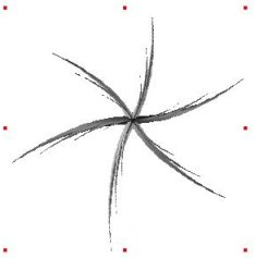
work as usual. The following figure illustrates a result obtained using
thick tubes as decorator, but it gives an idea of what could be
possible using flowers instead.

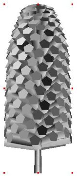
Object obtained using the golden ratio
option of the coil module
The second pane concerns
object distortion during the decoration
process. These distortions can only occur if :
- The decorator object is a TaPD object (tube or spline mesh)
- The decorator object is a planar spline mesh (leaf
distortion)
- The decorated object is a TaPD object (branching effects)
The figure
below shows the second pane.

Second pane of the coil module edit
window
The first series of
parameters address branch or leaf curving and bending. The case of
leaves is a bit special, so we'll ignore that one for now. As you have
seen from figure Coil.1, branches used to decorate a trunk remain
straight, which is most unlikely to happen in the case of real trees.
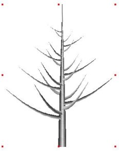
The Y
curvature angle is the angle towards which the branch tends, or
to be more precise the angle by which the branch will deviate from its
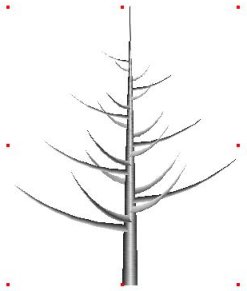
original orientation. If the vertical angle is 90° (as in figure
Coil.1), using a Y curvature angle of 40° yields figure Coil.2.a,
where the branches make a final vertical angle of 90°-40° =
50°. The default setting is such that branches follow a circle
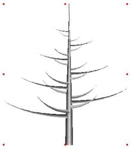
towards final orientation. This corresponds to a curvature rate
of 1. For some trees, however, branches are curved at the bottom and
then keep straight. A curvature rate greater than one simulate this
effect. A faster curvature is imposed at the bottom of the branch,
stopping when the specified
orientation is reached. Afterwards, the branch follows a straight line.
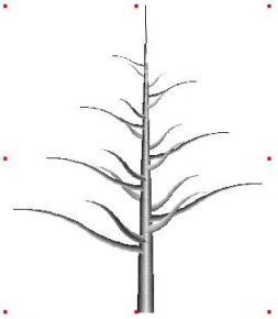
Figure coil.2.b illustrates this process using a Curvature rate of 2. Using rates
lower than 1, the opposite effect can be obtained : branches remain
straight near the trunk and then curve near the end to reach the
specified angular orientation. If you use low rates, it is likely that
the specified orientation is never reached simply because the process
slowed down too much. In that case, you can enter bigger values for the
curvature angle in order to reach the wished orientation.
As usual now, the +- parameter
allows to randomise the curvature angle, and the Y value button allows to vary the Y
curvature parameter along the Y axis of the decorated object. The
random distribution width is also sized using this function.

figure coil.2.a
Y curvature 40°, default curvature rate (1.0)
|

figure coil.2.b
Y curvature 40°,
curvature rate 2.0
|

figure coil.2.c
Y curvature 40°,
curvature rate 0.5
|
The Curve back to parameter
complicates the rules of the game evene more : it makes it possible to
get S shaped branches. When this parameter is non null, the Y curvature is applied to the first
half of the branch, twice the usual rate so that the orientation is
reached at the middle. At this point, the Curve back parameter is taken into
account, bending the branch the other way if this parameter is the
opposite sign of the Y curvature.
This design is illustrated in figure coil.3. However, you can use a Curve back parameter which has the
same sign as the Y curvature to design a special uniform shape of a
branch, if you wish to do so.
figure coil.3
Y curvature 40°,
Curve back to -40°
The
parameters of the R Curvature
work exactly the same way, except that the rotation axis is parallel to
the Y axis of the decorated object rather than perpendicular to it (see
figure Coil.4). This set of parameters are generally not of great use
to model trees. In plane motion of the branches is usually governed by
branching effects and random distorsion, see below. The Y value button scales all parameters
of this section (curvature angle, back curvature and random
distribution), except curvature rate.

figure coil.4
R curvature 40°,
seen from the top
Branching effects : When a big
branch departs from a trunk or a branch, it often happens that the
bearer deviates from its orientation, presumably due to a counter
reaction mechanical effect. The bearer usually recover the previous
orientation after a while. The angular tilt specifies by which angular
amount "plugging" a decorator object should deviate the decorated
object. The recover rate specifies at which rate the decorated object
should recover from the branching. It is usually a high rate, from 2 to
4 or 5. Presumably, branching effects decreases as the decorator
objects get smaller towards the top of the decorated object. For this
reason, the Y value customised
function default value starts at 1 at the bottom of the decorated
object to end at 0. The figure coil.5 illustrates a branching effect
obtained by plugging a single branch into a trunk. It also show that
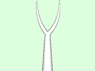
these parameters can be used to simulate trunk fork, which is not
possible otherwise in the TaPD at the moment.
Branching effects only work if the decorated object is a TaPD object.

figure coil.5
Using branching effects to simulate a trunk fork
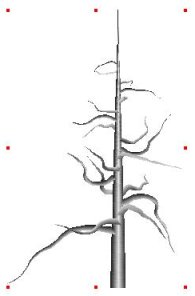
Random distortion : This parameter
works a bit like branching effects. What happens is that the shape of
some branches are like a lot of branching effects did occur, though no
branches are "plugged" at the point where the branch is distorted.
Maybe these branches fell, were cut or whatever. The random distortion
process starts to choose a random orientation and distorts the branch
accordingly. It then curve back the branch to its original orientation,
like the Curve back parameter
would do. The length of the branch affected is equal to the total
length divided by the number of random tilts to apply. The process is
repeated to the following segments using a new random orientation each
time. The Random tilt max angle
is the maximum angular amplitude that a random distortion can reach,
and the number of random tilts specifies how many segments of the
branch should be affected. The result is shown in figure Coil.4. You
can use this parameters for aquatic plants or evil-looking, gnarled
trees.

figure coil.6
Random distorsion using a max angle of 20° and 3 tilts
Cross-section effects : This section
is devoted to axial distortion of decorator objects. They can be
applied only if the object is a TAPD spline mesh object (the
cross-sections of tubes are circular by nature and cannot be
distorted). The first parameter, Cross-section
jitter, is the amount by which cross-section curves control
points are randomised along the radius. A value of 0.1, for example,
means that control-points will be placed anywhere between 90% and 110%
of their original radial length (taken from the center of the local
coordinate system of the curve to the control point). The result will
depend on how close in Y the cross-sections are (too close
cross-sections probably cancels out cross-section jitter) and the UV
smoothness of the spline mesh.
The twist parameters are used
to rotate cross-sections using the axis perpendicular to the
cross-section planes (Y axis). The first parameter specifies the
overall number of turns to impose to the object, and the second one is
the amount by which it should be randomised. Both parameters are float
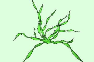
numbers and need not be integers. Twisting cross-sections and using
random distorsion described just above on a spline mesh object with
almost flat cross-sections, the following "aquatic plant like" object
was obtained :

figure coil.7
Using cross-section twist
Leaves special
section :
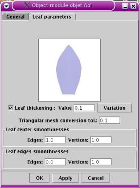
The coil module can also distort planar AoI spline meshes to obtain
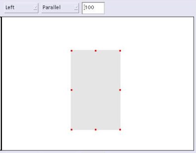
leaf distortion effects. The mesh must be created in AoI facing the
left direction (figure
Coil.8.a) for plants (leaves put on an a vertical stem) or the front direction for trees (leaves
put on horizontal branches or stems that departs from the main stem for
a plant ). After edition and shaping, an example of leaf
shape is shown on figure Coil.8.b. It is also possible to generate a
volumic triangular mesh out of this spline mesh using parameters in the
AoI object module edit window.

figure coil.8.a
|

figure coil.8.b
|
If this object
is imported into the TaPD and the corresponding AoI object is plugged
into a coil module, the parameters belonging to the second parameter
pane, distortion parameters,
are used to distort the leaf :

|
The Y curvature
parameter works as usual and bend the V axis of the leaf. The example
shown left results from a Y curvature of 40 and a back angle of -40.
|

|
The R curvature
parameter bends the U splines of the leaf. The example
shown left results from a R curvature of 40 and a back angle of -40
using normalised curvature. If
a random distribution is used, its component is calculated at each V
coordinate rather than once for the whole leaf.
|

|
The Random twist
parameter twists the leaf plane through rotations of the plane around
the V direction. The result for a maximum angle of 20° and a number
of twists of 3 is shown left.
|
Leaf
distortion has also a special section at the bottom of the pane to
specify special parameters that can't be expressed through use of the
parameters previously discussed.
The Leaf curvature angle
represents the in-plane distortion of the V or Y axis of the leaf. It
works exactly like other curvature angles discussed previously. The Y value function scales of the
curvature parameters. The figure below illustrates the leaf shpae
obtained with a leaf curvature of 30° and a back curvature of
-30° :
Leaf distortion
obtained with a leaf curvature of 30° and a back curvature of
-30°
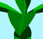
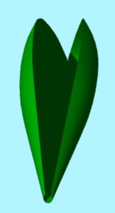
The Angle at center
parameter specifies the angle that makes a leaf about its V or Y axis.
This gives the leaf a V shape as illustrates the figures below :

Leaf distortion
obtained with an angle at center of 40°
The R curvature factor modifies the way
the R curvature is applied to the leaf. Basically, there are two
possibilities :
- The leaf
shape is constant across its length and varies along different widths,
like if it is was rolled around a tube. The small sections at the
beginning and the end of the leaf show small curvature, if not flat.
This scheme is called constant curvature.
- The
curvature is constant across the width of the leaf and vary along the
length. The small sections show the same shape as the main section of
the leaf, only scaled down. This scheme is called normalised curvature,
because it is normalised for each width of the leaf across its
length.
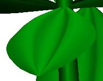
The R curvature factor slider allows to
choose any value between these two extremes. The figures below show
three leaves modeled using a R curvature angle of 70° in order to
exaggerate effects. The figure on the left uses a constant curvature
scheme. It looks much like a part of a tube surface, except for camera
distortion effects. The figure on the
right uses normalised curvature. With such a high
curvature angle, the spline mesh closes on itself like two parts of a
sea shell.


Three R curvature
values : constant curvature (left), normalised curvature (right) or
halway between the two (middle).
3.2.2 Golden
ball
module 

The golden ball
module paces object along the radii of a sphere following the golden
ratio rule. Its input and output ports are exactly the same as those of
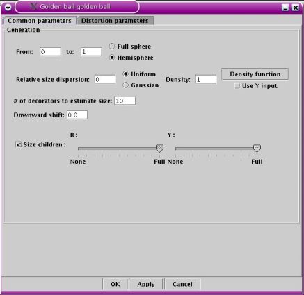
the coil module. The figure below whows the golden ball edit window :

Golden ball module
edit window
The Sphere and Hemisphere radio buttons specify if
the decoration geometry concerns a whole sphere or only half of it.
The from and to parameters specifies which part
of the sphere (or the hemisphere) should be considered. The process
starts from the top of the sphere at a coordinate of 0 ad ends at the
bottom for a coordinate of 1 for a sphere. The same considerations
apply to an hemisphere, except that the bottom is the disc section of
the half sphere. For example, using from and to values of 0.25 and 0.75
for a sphere means that the decoration process will happen in the
middle of it. A full hemispherical decoration is equivalent to using a
spherical decoration ranging from 0 to 0.5.
The Relative size dispersion
works exactly like in the coil module.
The Density parameter
represents how dense the packing of decorators is. The golden ball
module first calculate a density based on the R section of the
decorators, taking also into account any decoration process they might
have gone through. If this density is too small or too big (usually it
is to small for a close packing), you can increase/decrease it using
the density parameter.
The Density function button allows to
edit the customised function that specifies how density should vary
from the from parameter to the
to parameter. It is thus
possible to have a close packing at the start of the decoration process
and a loose packing at the end. The overall density used is the density
parameter multiplied by the value of the customised function at a given
point between from (origin of
the customised function) and to
(abscissae of one). Due to mathematical considerations, it is not
possible to ensure that an overall density that starts at 1 and ends at
2 gives the same result at the start than a decoration with a constant
density of 1 and at the end than a decoration
with a constant density of 2. Thus, It is likely that the density
parameter must be tuned to reach the wished result when using the
density function. The density function could be used to densify packing
when decorators get smaller due to the use of a size customised
function, for example.
Use Y input checkbox : As for the
coil module, this option makes it possible to use a value input in the
Y input port. The density is then constant (except when a random value
is input in the Y input port) and equal to the product of the density
parameter times customised function value calculated at the input value
coordinate.
The # of decorators to estimate
specifies how many decorators should be evaluated to estimate the
packing density. You can decrease this number if decorators have more
or less all the same size or increase it if the size varies a lot from
one decorator to the other.
Downward shift : by default, the
generated object is placed at the top of the decorated object. The downward shift allows to place it
anywhere along the height of the decorated object from the top
(downward shift = 0) to the bottom (downward shift = 1).
The Size children settings works exactly like in
the coil module.
The second pane allows for
distortion of the decorators object following the principles explained
in the coil module section.
Important
note : if the decorators show a very small section (very thin
tubes, for example), the density calculated by the golden ball module
might generate by default a huge number of objects, presumably causing
long computation time, if not an Out of Memory error. If you use
decorators with a tiny section, start with a low density
parameter, and increase as needed.
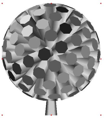
The following figure shows a result
obtained
using thick tubes as decorator :

A simple packing of
tubes
|

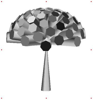
Hemispherical packing
of tube using a customised
size function plugged into the size inputs of the module
|
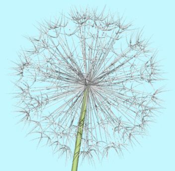
The dandelion flower shown below has been modeled using the golden ball
module. It is available in the example files. The dandelion flower
example and the principles of using the golden ratio to create a
spherical object is described in references [2] and [3].

A dandelion flower
modeled using the golden ball module
3.2.3 Top
module 

The top module
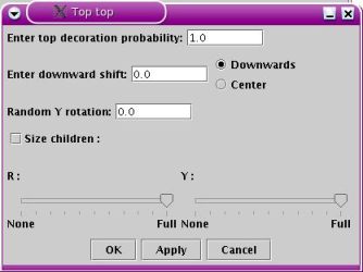
makes it possible to place the decorator object on top of the decorated
object. It is a simple geometry module. The edit window is shown below :

Top module edit window
The top decoration probability
is the probability that a decorator object gets placed on top of the
decorated object. The downward shift is the downwards translation
applied the decorator in reduced height of the decorated object. A
value of 0.05, for example, means that the decorator will be placed at
95% of the height of the decorated object. Using this parameter it is
possible to have a small overlap between the decorated object and the
decorator. Radio buttons allow to choose between Downwards, which the design which
has just been discussed, and Center.
If the Center radio button,
the decorator and decorated object centers are superimposed. For
example, this allows to place a light whithin a sphere. The Downward shift is ignored if the Center option is used.
The Random Y rotation allows
to rotate randomly the decorator object around the Y axis by a maximum
+- the value entered (in degrees). Using this parameter, it is possible
to avoid that flowers put on top of stems have all the same orientation
with respect to the Y axis.
The Size children function
works as for the coil module, see above.
3.2.4
Distort
module 

Using the coil
module, it is possible to distort the decorator objects given a set of
parameters. However, it is not possible to distort the decorated
object, except considering branching effects. The distort module makes
it possible to distort the decorated object as well. The edit window is
not shown here, it is a replica of the second pane of the coil module
edit window minus the branching effects parameters. The main use of the
Distort module is to distort a
starting object (say a trunk) before plugging it into a decoration
module. It can also be used to distort an object before plugging it as
decorator in a top module.
You should not plug the Distort module output into the
decorator input of a coil module. The distortion parameters of the coil
module will cancel any previous distortion carried out by the distort
module.
3.2.5 Random
module 

If an object
port output has multiple links, all the decoration processes
resulting from these links will be merged. Sometimes, however, it is
wished that one of these links should be chosen at random rather than
to have all the links results merged into a single decoration (these
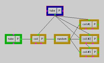
considerations are discussed at length in the next chapter). The figure
below illustrates a typical use of the Random
module :

Random module example
Whithout the random module inserted between the first coil module and
the other coil modules named #1 to #3, the three decorations
carried out by the three coil modules would be merged for each
decorator of the first coil module. Using the random module, however,
one of the #1, #2, #3 coil module is chosen for decorating each
decorator of the first coil module.
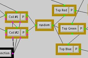
It is also possible to specify the probability of following a specified
output link. Let's consider the following example, taken from the lamp example file :

Random module used in
the lamp example
The default parameters of the random module are such that the
probabilities of decoration with a red, blue or green light are all
equal. Clicking the edit button brings this edit window :
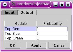
Random module edit
window
The tabbed pane consist in two tables, the input probabilities table
and the probabilities table. We will focus on the latter and suppose we
want twice as much blue lights than any other colour. Entering the
probabilities shown on the screenshot leads to such a situation. The
probabilities need not be integers or floats normalized to one, you can
use any scheme you wish (i.e. 0.25, 0.5, 0.25 or 1, 2, 1).
The other pane is devoted to input probabilities. This situation occur
if, for example, you plug three object modules into the input of a
random module and the output of the random module to the decorator
input port of a coil module. If you do not use the random module, the
default scheme is to choose as decorator one of the three objects at
random. If you use the random module, however, you will be able to
specify different probabilities for each one of the three objects.
The random process works either for the input port of the random module
or for its output port, depending on whether it is placed upstream
(random input) or downstream (random output). For upstream and
downstream definitions, see chapter 4.
Due to its function, the random module does not have a preview button.
3.3
Value modules
3.3.1
Constant value
module 

The constant
value module holds a float value, exactly like the procedural editor
value module. Its use is straightforward. One interest of the constant
value module is to plug it into one of the size entries of an object
module so that the size of the object can be quickly modified whithout
having to edit the object itself each time a size fine tuning is
required.
3.3.2
Customised function
module 

The customised
function module works exactly like the procedural editor customised
function (see AoI manual). Its main use is to be plugged into the coil
module size entries to vary the size of the decorator objects along the
Y axis of the decorated object. The editing window shows two additional
buttons, Copy function and Paste function that can be used to
copy and paste function control points and options between two editing
windows. These buttons can be used to replicate function definitions in
geometry modules like the coil module that makes heavy use of
customised functions.
3.3.3 Binary
operation module 

This module
takes two input values, named a
and b, and computes a result
r = f(a,b). The available operations not only include +, -, *, /, but
also <, >, Min, and Max. The type of operation performed is
selected in a combo box in the edit window, shown below. An illegal
operation like dividing by zero yields a zero value on output and an
error message in the console.

Binary operation edit
window
3.3.4 Unary
function module 

This module
takes one input value, named a,
and computes a result r = f(a). The available operations include abs,
exp, log, square root, sine and cosine. the sine and cosine are
normailzed to PI/2, ie. f(a) = sin(a*PI/2). The considered function is
selected in a combo box in the edit window,
shown below. An illegal operation like log(<=0) or sqrt(<0)
yields a zero
value on output and an error message in the console.

Unary function edit
window3.3.5
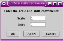
Scale/shift module 

This module,
identical to the one found in the procedural texture editor, takes one
input value and applies the
following linear transformation r = scale*a +shift. These two parameters
are entered in the edit window shown below.

Scale-shift module edit
window3.3.6
Clip
module 

The clip module
is also identical to the one found in the procedural texture editor. It
takes one input value and applies the
following rules
a < min -> r = min
min <= a <= max -> r = a
max <= a -> r = max
The min and max parameters are entered in the
edit window shown below.

Clip module edit
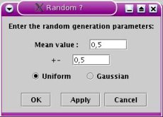
window3.3.7 Random
value module 

The random
value module delivers a random number following a random distribution
specified by the user. These parameters are the mean value of the
distribution and its spread. As for the coil module, two kinds of
distribution can be used : a uniform distribution and a gaussian
distribution. The edit window is shown below :

Random value edit
window


